What is Computer Programming?
Computer programming (a.k.a. programming) is the process of translating a predefined computer problem to a series of instructions that can be understood and processed by a CPU in order to provide a solution to the problem. In order for a computer program to be understood by the CPU the instructions must follow a particular syntax and the syntax used will be determined by the programming language(s) used to write the instructions.
Programming involves activities such as analysis, developing understanding, generating algorithms, verification of requirements of algorithms including their correctness and resources consumption, and implementation (commonly referred to as coding) of algorithms in a target programming language. Source code is written in one or more programming languages.
Throughout the evolution of computer programming many different paradigms and languages have been created to help organize and simplify the process.
Computer programming methodologies include:
- functional programming
- procedural programming
- imperative programming
- declarative programming
- object-oriented programming
- structural programming
The number of programming languages that have been developed over the history of computer programming have been numerous.
Some of the more popular programming languages include:
- Machine language
- Assembly language
- Fortran (1957) John Backus
- Algol (1958)
- Cobol (1959) Dr. Grace Murray Hopper
- Lisp (1959) John McCarthy (MIT)
- Basic (1964) John G. Kemeny and Thomas E. Kurtz
- Pacal (1970) Niklaus Wirth
- Smalltalk (1972) Alan Kaye, Adele Goldberg, and Dan Ingalls
- C (1972) Dennis Ritchie
- C++ (1983) Bjarne Stroustrup
- SQL (1972) Donald D. Cahmberlin
- Visual Basic (1991) Microsoft
- Python (1991) Guido Van Rossum
- Java (1995) Sun Microsystems
- PHP (1995) Rasmus Lerdorf
- C# (2000) Microsoft
- JavaScript (1995) Brendan Eich
Programming Paradigms
Functional Programming
According to Wikipedia, In computer science, functional programming is a programming paradigm where programs are constructed by applying and composing functions. It is a declarative programming paradigm in which function definitions are trees of expressions that map values to other values, rather than a sequence of imperative statements which update the running state of the program.
In functional programming, functions are treated as first-class citizens, meaning that they can be bound to names (including local identifiers), passed as arguments, and returned from other functions, just as any other data type can. This allows programs to be written in a declarative and composable style, where small functions are combined in a modular manner.
Functional programming is sometimes treated as synonymous with purely functional programming, a subset of functional programming which treats all functions as deterministic mathematical functions, or pure functions. When a pure function is called with some given arguments, it will always return the same result, and cannot be affected by any mutable state or other side effects. This is in contrast with impure procedures, common in imperative programming, which can have side effects (such as modifying the program's state or taking input from a user). Proponents of purely functional programming claim that by restricting side effects, programs can have fewer bugs, be easier to debug and test, and be more suited to formal verification.
Functional programming has its roots in academia, evolving from the lambda calculus, a formal system of computation based only on functions. Functional programming has historically been less popular than imperative programming, but many functional languages are seeing use today in industry and education, including Common Lisp, Scheme, Clojure, Wolfram Language, Racket, Erlang, Elixir, OCaml, Haskell, and F#. Functional programming is also key to some languages that have found success in specific domains, like JavaScript in the Web, R in statistics, J, K and Q in financial analysis, and XQuery/XSLT for XML. Domain-specific declarative languages like SQL and Lex/Yacc use some elements of functional programming, such as not allowing mutable values. In addition, many other programming languages support programming in a functional style or have implemented features from functional programming, such as C++, C#, Kotlin, Perl, PHP, Python, Go, Rust, Raku, Scala, and Java (since
Java 8).
Procedural Programming
According to Wikipedia, Procedural programming is a programming paradigm, derived from imperative programming, based on the concept of the procedure call. Procedures (a type of routine or subroutine) simply contain a series of computational steps to be carried out. Any given procedure might be called at any point during a program's execution, including by other procedures or itself. The first major procedural programming languages appeared circa 1957–1964, including Fortran, ALGOL, COBOL, PL/I and BASIC.[2] Pascal and C were published circa 1970–1972.
Imperative Programming
In computer science, imperative programming is a programming paradigm that uses statements that change a program's state. In much the same way that the imperative mood in natural languages expresses commands, an imperative program consists of commands for the computer to perform. Imperative programming focuses on describing how a program operates.
The term is often used in contrast to declarative programming, which focuses on what the program should accomplish without specifying how the program should achieve the result.
Declarative Programming
In computer science, declarative programming is a programming paradigm—a style of building the structure and elements of computer programs—that expresses the logic of a computation without describing its control flow.
Many languages that apply this style attempt to minimize or eliminate side effects by describing what the program must accomplish in terms of the problem domain, rather than describe how to accomplish it as a sequence of the programming language primitives (the how being left up to the language's implementation). This is in contrast with imperative programming, which implements algorithms in explicit steps.
Declarative programming often considers programs as theories of a formal logic, and computations as deductions in that logic space. Declarative programming may greatly simplify writing parallel programs.
Common declarative languages include those of database query languages (e.g., SQL, XQuery), regular expressions, logic programming, functional programming, and configuration management systems.
Object Oriented Programming
According to Wikipedia, Object-Oriented Programming (OOP) is a programming paradigm based on the concept of "objects", which can contain data and code. The data is in the form of fields (often known as attributes or properties), and the code is in the form of procedures (often known as methods).
Structural Programming
Structured programming is a programming paradigm aimed at improving the clarity, quality, and development time of a computer program by making extensive use of subroutines, block structures, for and while loops—in contrast to using simple tests and jumps such as the go to statement, which could lead to "spaghetti code" that is difficult to follow and maintain.
It emerged in the late 1950s with the appearance of the ALGOL 58 and ALGOL 60 programming languages, with the latter including support for block structures. Contributing factors to its popularity and widespread acceptance, at first in academia and later among practitioners, include the discovery of what is now known as the structured program theorem in 1966, and the publication of the influential "Go To Statement Considered Harmful" open letter in 1968 by Dutch computer scientist Edsger W. Dijkstra, who coined the term "structured programming".
Structured programming is most frequently used with deviations that allow for clearer programs in some particular cases, such as when exception handling has to be performed.
More on Structured Programming (Wikipedia)
Which Programming Language Should I Learn First?
If it were me, I would go with C# first. However, the problem with C# in academia is that four-year universities hate Bill Gates due to an open letter he wrote in the late 70’s telling personal computer hobbyists to stop stealing his BASIC code. This negative attitude prevails today and has been institutionalized in universities by preventing C# from being a transferable course for their Computer Science degrees. This is why community colleges only offer C# classes infrequently, if at all; it doesn’t always get enough enrollment due to the fact that it is not transferable to the four-year universities.
I’m not a fan of C++, I feel it is antiquated compared to C#, Java, and Python. That said, when compiled, C++ usually runs faster than the others when compared head-to-head and is better suited for getting closest to the computer hardware. Thus making it a better choose for writing operating systems, hardware drivers, and complex gaming systems. C++ is a derivative of the original C language family which includes C# and Java, making C# and Java easier to learn once you have learned to write software with C++.
Python is considered to be easier than all of them to learn, but it is not part of the C family of programming languages, thereby it is uses quite different programming structures than the others. As mentioned previously, learning C++ will make it much easier to learn C# and Java. Eventually, you will want/need to learn more than one programming language – making you a polyglot. A lot of beginning programming students take the easy route and learn Python which is used mainly in data analysis, analytics, and AI. but I recommend the C languages as they are more widely used in most computer programming jobs.
I hope this gives you a good foundation for choosing which programming language to learn first.
Anatomy of a Computer Program
A computer program is a collection of precise instructions to complete a task. In order to help determine which tasks a computer program needs to accomplish and the instructions required to complete those tasks, a certain amount of analysis and design needs to occur before the programmer can begin the development, testing, and implementation of a computer program.
Earlier in this course you learned about the software development life cycle, in this section you will examine the software design step in greater depth.
Designing a Solution
Before a computer program can be written, first the specifications of the program need to be documented. In addition to specifying the input(s) and the output, the steps necessary to convert the input into the correct ouput also need to be defined. In the following video the presenter demonstrates how computer programmers go about defining and documenting a simple problem, giving directions on how to get from point A to point B.
This video the demonstrates the concept of an alogrithm using the example of giving someone driving directions to get to a specific destination.
⇑ Table of Contents
Introducing Algorithms
An algorithm is a well-ordered collection of unambiguous and effectively computable operations that, when executed, produces a result and halts in a finite amount of time.
During the design phase of developing a computer program each task that the program must perform is broken down into a series of logical steps. These steps are commonly represented by Pseudocode, Flowcharts, and/or Decision Tables. The image below shows another example of an algorithm, how to prepare a dessert. The step-by-step instructions for how to prepare the dessert are the algorithm in this example.
Algorithm for Making Rich Chocolate Pudding
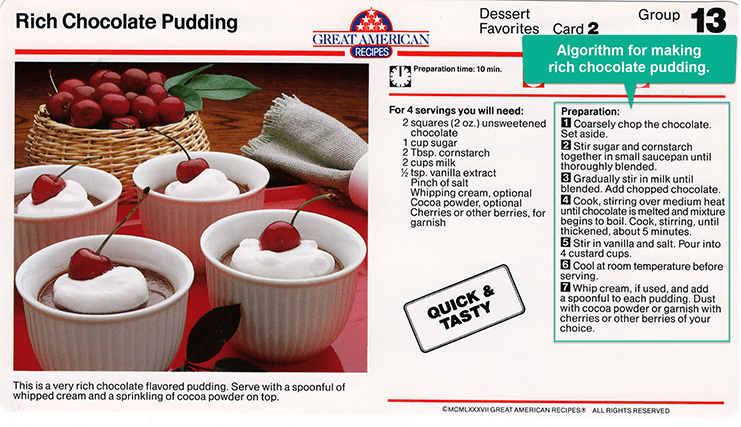 Figure 1
Algorithm for Programming Your DVR
| Step 1 |
If the clock and the calendar are not correctly set, then go to page 9 of the instruction manual and follow the instructions there before proceeding to Step 2 |
| Step 2 |
Repeat Steps 3 through 6 for each program that you want to record |
| Step 3 |
Enter the channel number that you want to record and press the button labeled CHAN |
| Step 4 |
Enter the time that you want recording to start and press the button labeled TIME-START |
| Step 5 |
Enter the time that you want recording to stop and press the button labeled TIME-FINISH. This completes the programming of one show |
| Step 6 |
If you do not want to record anything else, press the button labeled END-PROG |
| Step 7 |
Turn off your DVR. Your DVR It is now in TIMER mode, ready to record |
⇑ Table of Contents
Once we have formally specified an algorithm, we can build a machine (or write a program or hire a person) to carry out the steps contained in the algorithm. The machine (or program or person) need not understand the concepts or ideas underlying the solution. It merely has to do Step 1, Step 2, Step 3, . . . exactly as written. In computer science terminology, the machine, robot, person, or thing carrying out the steps of the algorithm is called a computing agent.
“. . . a well-ordered collection . . .”
An algorithm is a collection of operations, and there must be a clear and unambiguous ordering to these operations. Ordering means that we know which operation to do first and precisely which operation to do next as each step is successfully completed. After all, we cannot expect a computing agent to carry out our instructions correctly if it is confused about which instruction it should be doing next.
Consider the following “algorithm” that was taken from the back of a shampoo bottle and is intended to be instructions on how to use the product.
Algorithm for Washing Your Hair
Step 1: Wet hair
Step 2: Lather
Step 3: Rinse
Step 4: Repeat
At Step 4, what operations should be repeated? If we go back to Step 1, we will be unnecessarily wetting our hair. (It is presumably still wet from the previous operations.) If we go back to Step 3 instead, we will not be getting our hair any cleaner because we have not reused the shampoo. The Repeat instruction in Step 4 is ambiguous in that it does not clearly specify what to do next. Therefore, it violates the well-ordered requirement of an algorithm. (It also has a second and even more serious problem—it never stops! We will have more to say about this second problem shortly.) Statements such as:
-
Go back and do it again. (Do what again?)
-
Start over. (From where?)
-
If you understand this material, you may skip ahead. (How far?)
-
Do either Part 1 or Part 2. (How do I decide which one to do?)
are ambiguous and can leave us confused and unsure about what operation to do next. We must be extremely precise in specifying the order in which operations are to be carried out. One possible way is to number the steps of the algorithm and use these numbers to specify the proper order of execution. For example, the ambiguous operations just shown could be made more precise as follows:
-
Go back to Step 3 and continue execution from that point.
-
Start over from Step 1.
-
If you understand this material, skip ahead to Line 21.
-
If you are 18 years of age or older, do Part 1 beginning with Step 9; otherwise, do Part 2 beginning with Step 40
“ . . .of unambiguous and effectively computable operations. . .”
Algorithms are composed of things called “operations,” but what do those operations look like? What types of building blocks can be used to construct an algorithm? The answer to these questions is that the operations used in an algorithm must meet two criteria—they must be unambiguous, and they must be effectively computable.
Here is a possible “algorithm” for making a cherry pie:
Algorithm for Making a Cherry Pie
Step 1: Make the crust
Step 2: Make the cherry filling
Step 3: Pour the filling into the crust
Step 4: Bake at 350°F for 45 minutes
For a professional baker, this algorithm would be fine. He or she would understand how to carry out each of the operations listed. Novice cooks, like most of us, would probably understand the meaning of Steps 3 and 4. However, we would probably look at Steps 1 and 2, throw up our hands in confusion, and ask for clarification. We might then be given more detailed instructions.
Algorithm for Making a Cherry Pie (alt.)
- Step 1: Make the crust
- Take one and one-third cups flour
- Sift the flour
- Mix the sifted flour with one-half cup butter and one-fourth cup water
- Roll into two 9-inch pie crusts
- Step 2: Make the cherry filling
- Open a 16-ounce can of cherry pie filling and pour into bowl
-
- Add a dash of cinnamon and nutmeg, and stir
With this additional information, most people—even inexperienced cooks—would understand what to do and could successfully carry out this baking algorithm. However, there might be some people, perhaps young children, who still do not fully understand each and every line. For those people, we must go through the simplification process again and describe the ambiguous steps in even more elementary terms.
For example, the computing agent executing the algorithm might not know the meaning of the instruction “Sift the flour” in Step 1.2, and we would have to explain it further.
| 1.2 |
Sift the flour
1.2.1 Get out the sifter, which is the device shown on page A-9 of your cookbook, and place it directly on top of a 2-quart bowl
1.2.2 Pour the flour into the top of the sifter and turn the crank in a counter-clockwise direction
1.2.3 Let all the flour fall through the sifter into the bowl |
Now, even a child should be able to carry out these operations. But if that were not the case, then we would go through the simplification process yet one more time, until every operation, every sentence, every word was clearly understood.
An unambiguous operation is one that can be understood and carried out directly by the computing agent without further simplification or explanation. When an operation is unambiguous, we call it a primitive operation, or simply a primitive of the computing agent carrying out the algorithm. An algorithm must be composed entirely of primitives. Naturally, the primitive operations of different individuals (or machines) vary depending on their sophistication, experience, and intelligence, as is the case with the cherry pie recipe, which varies with the baking experience of the person following the instructions. Hence, an algorithm for one computing agent might not be an algorithm for another.
One of the most important questions we will answer in this text is, what are the primitive operations of a typical modern computer system? Which operations can a hardware processor “understand” in the sense of being able to carry out directly, and which operations must be further refined and simplified?
However, it is not enough for an operation to be understandable. It must also be doable by the computing agent. If an algorithm tells me to flap my arms really quickly and fly, I understand perfectly well what it is asking me to do. However, I am incapable of doing it. “Doable” means there exists a computational process that allows the computing agent to complete that operation successfully. The formal term for “doable” is effectively computable.
For example, the following is an incorrect technique for finding and printing the 100th prime number. (A prime number is a whole number not evenly divisible by any numbers other than 1 and itself, such as 2, 3, 5, 7, 11, 13, ...)
Algorithm for Finding and Printing the 100th Prime Number
Step 1: Generate a list L of all the prime numbers: L1, L2, L3, . . .
Step 2: Sort the list L into ascending order
Step 3: Print out the 100th element in the list, L100
Step 4: Stop
The problem with these instructions is in Step 1, “Generate a list L of all the prime numbers....” That operation cannot be completed. There are an infinite number of prime numbers, and it is not possible in a finite amount of time to generate the desired list L. No such computational process exists, and the operation described in Step 1 is not effectively computable.
Additional Examples of Operations That May Not Be Computable
Case 1: Set number to 0.
Set average of number. (Division by 0 is not permitted.)
Case 2: Set N to -1.
Set the value of result to √N. (You cannot take the square root of negative values using real numbers.)
Case 3: Add 1 to the current value of x. (What if x currently has no value? Attempting to increment or dcrement declared but not initialized variables will result in a "use of unassigned local variable" error.)
. . .that produces a result. . .
Algorithms solve problems. To know whether a solution is correct, an algorithm must produce an observable result to a user, such as a numerical answer, a new object, or a change to its environment. Without some observable result, we would not be able to say whether the algorithm is right or wrong or even if it has completed its computations. In the case of the DVR algorithm (Figure 1.1), the result will be a set of recorded TV programs. The addition algorithm (Figure 1.2) produces an m-digit sum.
Note that we use the word result rather than answer. Sometimes it is not possible for an algorithm to produce the correct answer because for a given set of input, a correct answer does not exist. In those cases, the algorithm may produce something else, such as an error message, a red warning light, or an approximation to the correct answer. Error messages, lights, and approximations, although not necessarily what we wanted, are all observable results.
. . .and halts in a finite amount of time.
Another important characteristic of algorithms is that the result must be produced after the execution of a finite number of operations, and we must guarantee that the algorithm eventually reaches a statement that says, “Stop, you are done” or something equivalent. We have already pointed out that the shampooing algorithm was not well ordered because we did not know which statements to repeat in Step 4. However, even if we knew which block of statements to repeat, the algorithm would still be incorrect because it makes no provision to terminate. It will essentially run forever, or until we run out of hot water, soap, or patience. This is called an infinite loop, and it is a common error in the design of algorithms.
Solution To Washing Hair Problem
| Step |
Operation |
| 1 |
Wet your hair |
| 2 |
Set the value of WashCount to 0 |
| 3 |
Repeat steps 4 through 6 until the value of WashCount equals 2 |
| 4 |
Lather you hair |
| 5 |
Rinse your hair |
| 6 |
Add 1 to the value of WashCount |
| 7 |
Stop, you have finished shampooing your hair |
Figure 1.3 shows an algorithmic solution to the shampooing problem that meets all the criteria discussed in this section if we assume that you want to wash your hair twice. The algorithm of Figure 1.3 is well ordered. Each step is numbered, and the execution of the algorithm unfolds sequentially, beginning at Step 1 and proceeding from instruction i to instruction i 1 1, unless the operation specifies otherwise. (For example, the iterative instruction in Step 3 says that after completing Step 6, you should go back and start again at Step 4 until the value of WashCount equals 2.) The intent of each operation is (we assume) clear, unambiguous, and doable by the person washing his or her hair. Finally, the algorithm will halt. This is confirmed by observing that WashCount is initially set to 0 in Step 2. Step 6 says to add 1 to WashCount each time we lather and rinse our hair, so it will take on the values 0, 1, 2, . . . However, the iterative statement in Step 3 says stop lathering and rinsing when the value of WashCount reaches 2. At that point, the algorithm goes to Step 7 and terminates execution with the desired result: clean hair. (Although it is correct, do not expect to see this algorithm on the back of a shampoo bottle in the near future.)
As is true for any recipe or set of instructions, there is always more than a single way to write a correct solution. For example, the algorithm of Figure 1.3 could also be written as shown in Figure 1.4. Both of these are correct solutions to the shampooing problem. (Although they are both correct, they are not necessarily equally elegant.
Algorithmic Origins
Introducing Pseudocode
One simple way to write out a program's logic is to break each task that the program must perform into a series of logical steps. Using the example in figure 2 which is a flowchart representing a program that compares two numbers and outputs the larger of the two, you might write out the steps in this fashion:
- Input the first number and assign it to variable x
- Input the second number and assign it to variable y
- Compare the value of x to y
- If the value of x is greater than the value of y, display the value of x
- If the value of y is greater than the value of x, display the value of y
This is an example of an algorithm written in pseudocode. It is not written out in any particular programming language, but it can be used as a starting point for writing the actual programming code.
Introducing Flowcharts
A flowchart is a graphical representation of an algorithm. Figure 1 shows commonly used flowchart symbols available in the Microsoft Visio program. In figure 2 you see an algorithm designed to compare two numbers and display the larger of the two. Flowcharts can also be helpful to application developers in thinking through how an algorithm will be implemented in code.
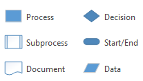 Figure 1: Standard flowchart symbols available in Microsoft Visio.
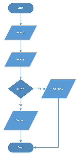 Figure 2: An example of a flowchart showing the necessary steps to complete a number comparison algorithm.
Introducing Decision Tables
Decision tables are a precise yet compact way to model complex rule sets and their corresponding actions. Decision tables are usually represented in coding structures as a series of if-else statements or a switch block.
Decision tables are made up of four quadrants: conditions, condition alternatives, actions, and action entries.
- Conditions represent under what condition an action should be applied.
- Condition alternatives are boolean values indicating which action entries apply or don't apply
- Actions indicate one or more actions to apply
- Action entries are values or check-marks indicating what value to apply or in the case of multiple actions, check-marks indicating which actions apply.
In this example (figure 3), the decision table represents an algorithm for calculating discounts based on the quantity of product purchased. If the buyer purchases less than 10 items they will receive a 5% discount, if they purchase between 10 to 49 items they will receive a 10% discount, if they purchase 50 to 99 items they will get a 15% discount, and any purchase of 100 or more items will result in a 20% discount.
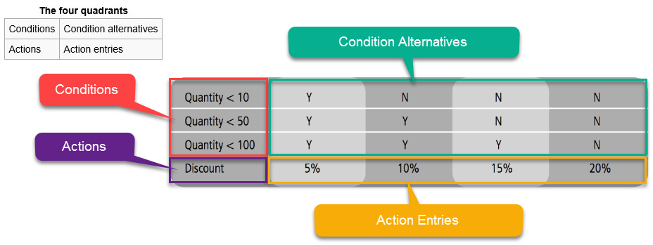 Figure 3: A decision table dissected into its four constituent parts: conditions, condition alternatives, actions, and action entries.
We'll have a chance to write this Decision Table out as actual C# code at the end of this lesson. First, you need to learn some basics about integrated development environments (IDEs) and how to use them to write a computer program.
⇑ Table of Contents
Variables
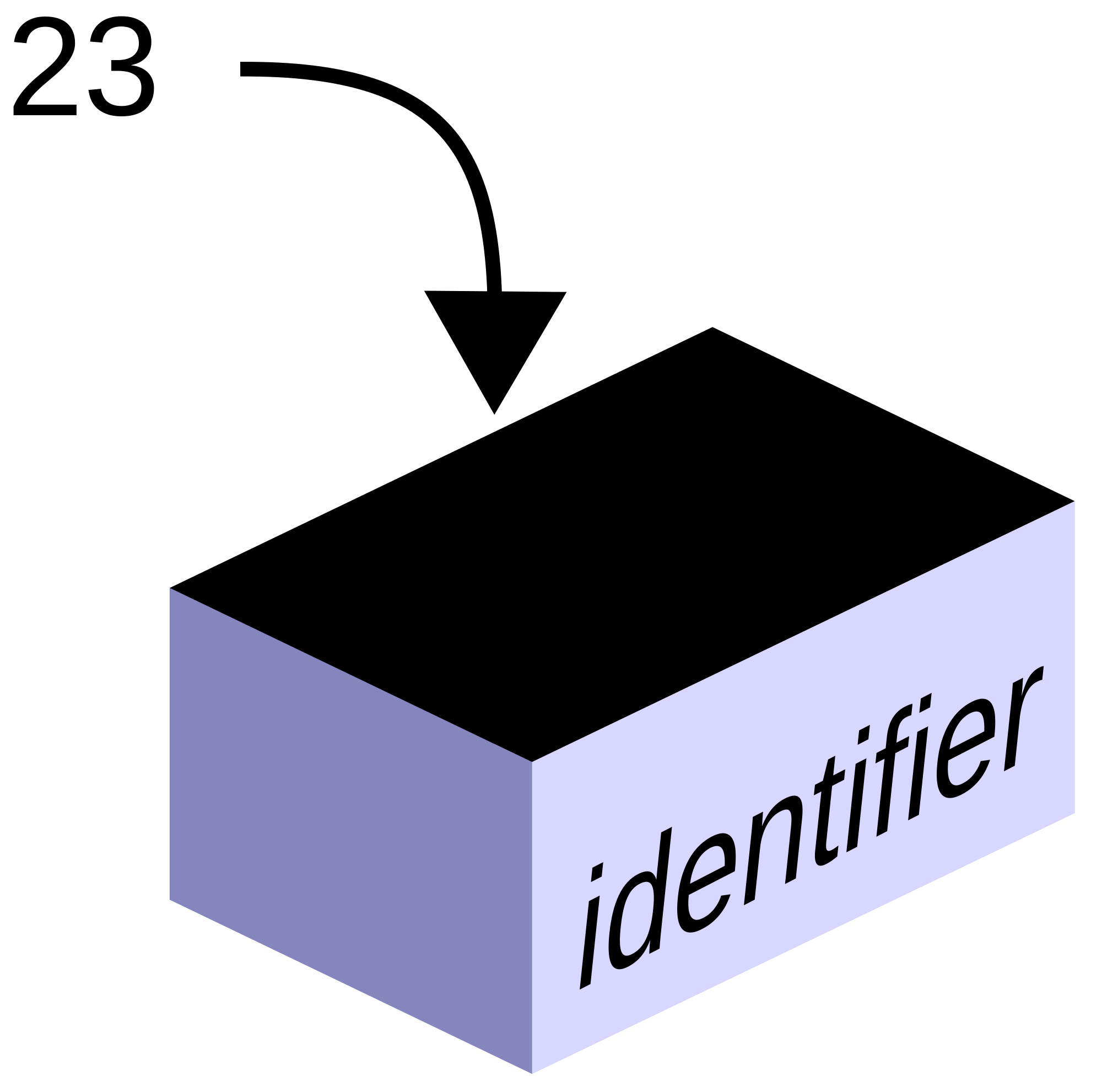 Figure 1: Conceptual representation of a variable.
Variables are a way of creating a temporary area of storage in computer memory for storing data while a program is running. Variables are named storage locations that hold values. We can then retrieve the value stored in memory by using the name (a.k.a. identifier) we assign to it when declaring the variable. Think of a variable as a placeholder or a box of a specific size which we can write a name on to help us to recall the data programmatically at a later time. For instance let's declare a variable named age and then later we'll store a value in it.
To do this we must follow the C# required format, data-type name; like this:
int age;
In the C# language we are required to include one of the C# data types provided by the .NET framework to let the compiler know what kind of value it should expect when we assign a value to it. The data type also determines what kinds of operations can be performed on it. In our example we used int which represents a 32-bit value which can only be a whole number, either positive or negative. By informing the compiler that our variable will be used to store a 32-bit integer value, the compiler now knows how many bits of space it needs to reserve in memory for holding the value when we assign data to it. You can determine a C# variable's data type like this variable_name.GetType();
Should we forget and try to assign text as a value for our variable or another numeric data type like a float data type, say 23.5, the compiler will let us know that this is not allowed while we are writing our program instead of us finding out the hard way, later on after the program has been compiled and being run by our customer. This saves a lot of time and
money.
For more information on the data types available for use in the C# language, read the section titled Data Types.
You can also initialize our variable (assign a value to it) at the same time we declare it by adding the C# assignment operator (=) followed by a value, like this:
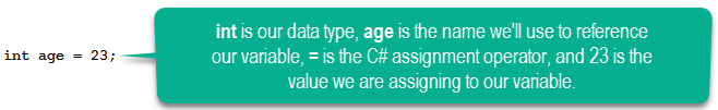
Notice how asignment goes from right to left. Whether you are initializing a variable or just modifying its current value, assignments always go from right to left. Once our variable is declared or initialized, we can change the value of our variable at any time by simply writing an assignment statement using the name of the variable, the assignment operator, and a new value, like this:
    //variable = expression
    age = 45;
variable names must start with a letter or an underscore and can contain only letters, numbers, or underscores. A variable name can only be a maximum of 255 characters and must be unique within scope (more on local and global variables [scope] later).
Beginning in Visual C# 3.0, variables that are declared at method scope can have an implicit type var. An implicitly typed local variable is strongly typed just as if you had declared the type yourself, but the compiler determines the type. The following two declarations of i are functionally equivalent:
        var i = 10; //implicitly typed
        int i = 10; //explicitly typed
Python is a dynamically typed language like JavaScript in that the interpreter infers the data type at run-time based on the value assigned to the variable. For instance, age = 20 would give the inference that age is an int. However, if we declare age like this age = "20" then the inference is that age should be a string type. You can test this in Python using the type() function, like this: type(variable_name).
In JavaScript the keyword var is used to dynamically declare a variable's data type, for example: var age = 20;. When the var keyword is not used in the declaration of a JavaScript variable, the variable is considered global in scope even if the declaration appears inside of a structure like a for loop.
Creating Variables
⇑ Table of Contents
Constants
Constants are immutable values which are known at compile time and do not change for the life of the program. Constants are declared with the const modifier. Only the C# built-in types (excluding System.Object) may be declared as const. Example:
const int i = 20;
In this example a constant named i is declared which stores an integer data type of the value 20. Once declared the value of the const cannot be changed.
Python and JavaScript do not have the concept of a constant, instead global variables in which values cannot be changed are used instead.
⇑ Table of Contents
Values
A value is a discrete quantity of data. The members of a type are the values of that type. Computer languages vary in their implementation of primitive value types, but some examples would be null, undefined, true/false, and numeric values, like the following: 1, 3.1459, "Chuck", 'D', true.
Data Types
A data type or simply type is a classification of data which tells the compiler or interpreter how the programmer intends to use the data. Data types specify the type of data that you work with in a program. The data type defines the size of memory needed to store data and the kinds of operations that can be performed on the data. Most computer programming languages support various types of data, for example: real, integer, string, or boolean. A data type provides a set of values from which an expression (i.e. variable, function...) may take its values. The type defines the operations that can be done on the data, the meaning of the data, and the way values of that type can be stored. Data types are grouped into value types and reference types. Value data types store the value on the stack, whereas reference data types write the memory address on the stack which
points to where the data value begins in dynamic memory (the heap).
Modern-day programming languages have basic data types built-in to them; these are generally referred to as their primitive data types. Meaning, the programmer does not have to write the code that defines the data type, its allowed operations, etc. Usually a simple statement like:
int myVariable;
is all that is needed to declare an integer variable to the compiler or interpreter using any modern-day programming language.
Data Types By Programming Language
Click on the links below to view the specific data types for the designated programming language.
C++ Fundamental Types
C++ Fundamental Types (official documentation)
Data types in C++ are mainly divided into two types:
Primitive Data Types: These data types are built-in or predefined data types and can be used directly by the user to declare variables. example: int, char , float, bool etc. Primitive data types available in C++ are:
- Integer
- Character
- Boolean
- Floating Point
- Double Floating Point
- Valueless or Void
- Wide Character
Abstract or user defined data type: These data types are defined by user itself. Like, defining a class in C++ or a structure.
JavaScript Built-In Data Types
JavaScript Built-In Data Types (official documentation)
In JavaScript, a primitive (primitive value, primitive data type) is data that is not an object and has no methods. There are 6 primitive data types: string, number, boolean, null, undefined, symbol (new in ECMAScript 2015).
Most of the time, a primitive value is represented directly at the lowest level of the language implementation.
All primitives are immutable, i.e., they cannot be altered. It is important not to confuse a primitive itself with a variable assigned a primitive value. The variable may be reassigned a new value, but the existing value can not be changed in the ways that objects, arrays, and functions can be altered.
Java Data Types
Java Data Types (official documentation)
The Java programming language supports the following primitive data types.
- byte
- short
- int
- long
- float
- double
- boolean
- char
Notice that the Java primitive data tyes all begin with a lowecase character. This format indicates that the data type is a primitive type, meaning that it defines the size that will be reserved in memory for that data type, but it has no associated methods. Java also has data type objects which in addition to defining the size of the data type they also have associated methods which allow for manipulation of the data type. Java object data type names are the same as the primitive type names except that they begin with a capital letter, e.g. Byte, Int, Double, etc.
Python Built-In Types
Python Built-In Types (official documentation)
Python has four primitive data types:
- Integers
- Float
- Strings
- Boolean
C# Data Types
C# Data Types (official documentation)
C# provides several built-in data types by way of the .NET framework which can be used in your programs. You can also define new data types by defining your own data structure, such as a class or a struct.
In this lesson we focus on some of the most commonly used data types.
Figure 2: C# Data Types
| Data Type |
Size |
Range Of Values |
| byte |
1 byte |
0 to 255 |
| char |
2 bytes |
U+0000 to U+ffff (Unicode characters) |
| short |
2 bytes |
-32,768 to 32,767 |
| int |
4 bytes |
-2,147,483,648 to 2,147,483,647 |
| long |
8 bytes |
-9,223,372,036,854,775,808 to 9,223,372,036,854,775,807 |
| float |
4 bytes |
±1.5 X 10-45 to ±3.4 X 1038 |
| double |
8 bytes |
±5.0e-324 to ±1.7e308 |
| bool |
2 bytes |
True or False |
| string |
- |
zero or more unicode characters |
All of the data types in the table above are value types except for string, which is a reference type. The variables which are based on value types directly contain the value on the stack. Data types which are of type reference store a reference on the stack which points to a memory address on the heap where the value is actually stored. This will make more sense after you learn about arrays, stacks, heaps, and other data structures later on in this course. For now, just remember that the string type is a reference type and NOT a value type.
The MSDN Web site has a more comprehensive table showing the C# integral data types. which is a subset of the simple types. You might also want to review Types for a more comprehensive overview of C# types.
⇑ Table of Contents
Operators
You have already seen a couple of C# operators in action (= and new). In this section we will discuss C# operators in more depth.
Operators are symbols that specify which operations (math, indexing, function call, etc.) to perform on the operands in an expression. Operands can be variables, constants, literals, etc. Operators can be organized by function or by number of operands it operates on. If we organize operators by function, each operator would fall into one of three categories, 1) arithmetic, 2) boolean, or 3) relational. Examples of arithmetic operators include: +, -, *, /, and %. If we organize operators by the number of operands they operate on then the groupings would be: 1) unary operators, 2) binary operators, and 3) ternary operators.
Operators can be organized depending on the number of operands involved, like this:
Unary operators: The unary operators work with only one operand. Examples include ++x (prefix increment), x++ (postfix increment), or new.
Binary operators: Binary operators take two operands. Examples include x + y or x > y
Ternary operators: Ternary operators take three operands. There is just one ternary operator in C# ?:. Pseudo code example:
condition ? expression_if_true : expression_if_false;
Operators can also be organized by how they are used, like this:
Arithmetic operators can be used to create expressions like:
x = 1 + 1;
Conditional operators can be used to create expressions like:
if (x < 2)
Logical operators can be used to create expressions like:
if (x<2 && y == 3)
Often expressions involve more than one operator. In this case the compiler needs to determine which operator takes precedence over the other(s). Figure 3 lists the C# operators in order of precedence (pretty much the same in all computer programming languages). The higher an operator is located in the table, the higher the precedence. Operators with higher precedence are evaluated before operators with lower precedence. Operators that appear in the same row have equal precedence.
Figure 3: C# Operators
| Category |
Operators |
| Primary |
x.y f(x) a[x] x++ x-- new
typeof checked unchecked |
| Unary |
+ - ! ~ ++x --x (T)x |
| Multiplicative |
* / % |
| Additive |
+ - |
| Shift |
<< >> |
| Relational and type testing |
<> <= >= is as |
| Equality |
== != === !== |
| Logical AND |
& |
| Logical XOR |
^ |
| Logical OR |
| |
| Conditional AND |
&& |
| Conditional OR |
|| |
| Conditional ternary |
?: |
| Assignment |
= *= /= %= += -= <<= >>= ^= |= |
The unary increment operator (++) adds 1 to the value of the an identifier (variable). Similarly, the decrement (--) operator subtracts 1 from the value of the identifier. The unary increment and decrement operator can be used as prefixes or suffixes. For example:
int x = 10;
x++; //value of x is now 11
++x; //value of x is now 12
However, when used as part of an assignment the results can be unexpected. When the unary increment and decrement operators are used as prefixes (++x), the current value of the identifier is returned after (post) the increment or decrement operation. When used as a suffix (x++), the value of the identifier is returned before (pre) the increment decrement operation is complete. To better understand how this works let's look at another example:
int x = 10;
int y = x++ //value of y is 10 (assigned pre-increment)
int z = ++x //value of z is 12 (assigned post-increment)
In this example, because y is assigned the value of x pre-increment y's value is 10. However x is increment after the assignment to y so x's value is now 11. Then, z is assigned the value of x post-increment so both x and y now have the value of 12. Fun stuff, eh?
If this example boggles you brain, I encourage you to copy this console application code into Visual Studio and try it out for yourself:
using System;

namespace IncrementDecrementOperators
{
    class Program
    {
        static void Main(string[] args)
        {
            int x = 10;
            int y = x++; //value of x is now 11
            Console.WriteLine("x = " + x + ", y = " + y);
            int z = ++x; //value of x is now 12
            Console.WriteLine("x = " + x + ", z = " + z);
        }
    }
}
Assignment, Comparison, and Logical Operators
Addition Vs. Concatenation
⇑ Table of Contents
Programming Principles
The Hollywood Principle
"Don't Call Us, Well Call You"
The DRY Principle
Don't Repeat Yourself
The Dependency Inversion Principle
High level modules should not depend on low level modules; both should depend on abstractions. Abstractions should not depend on details. Details should depend upon abstractions.
BBoM
Foote and Yoder use the term "Big Ball of Mud" (BBoM) to describe an application that appears to have no distinguishable architecture (think big bowl of spaghetti versus dish of layered lasagna). The issue with allowing software to dissolve into a BBoM becomes apparent when routine changes in workflow and small feature enhancements become a challenge to implement due to the difficulties in reading and understanding the existing codebase.
Understanding Arrays
In any programming language, C# included, an array is used to represent a collection of items; e.g. student test scores, a list of names, days of the week, etc. An array is a data structure that contains a number of variables called the elements of the array. The array elements are accessed through computed indexes. C# arrays are zero-based; meaning, all array indexes start at zero. All of the array elements must be of the same type, which is called the element type of the array. Array elements can be of any type, including an array type. An array can be a single-dimensional array, or a multidimensional array. Array types are reference types derived from the abstract base type System.Array.
Here are two examples of C# statements declaring and initializing a single-dimensional array:
int[] numbers = new int[5];
int[] numbers = {1, 2, 3, 4, 5};
In the first example, a single-dimensional array of integers called numbers is created. The array declaration begins with the array's element type, that is the type of data that will be stored in the array. The element type is followed by a pair of square brackets indicating we want to create an array. To the right of the assignment operator, the new operator followed by the rank specifier (how many elements to create in the array) encapsulated in square brackets is used to create the array and initialize the array elements to their default values. In this example, all the array elements are initialized to zero and the array contains 5 elements from array[0] to array[4].
In the second example, after the assignment operator, instead of using the new operator, a list of values we want to store in the array are encapsulated inside a set of curly braces. Just like any C# declaration both examples end with a semi-colon. Any of the array's elements can be directly accessed by using its index value. For instance, using the second example, we could retrieve the value of the second element in numbers by writing numbers[1]. Remember, array indexes begin at 0 meaning element 1 is index [0] making element 2's index value [1] and it is illegal to try an access an array's index outside of its range, meaning numbers[5] will throw an error because [4] is the last index in the example 2 array.
Also, just like we saw with variables, an array can be declared without initializing it with any values - like this:
int[] numbers;
For more examples of single-dimensional arrays see the C# Programming Guide.